Calculating Distance and Bearing Between Two Coordinates
Author: Sercan Fidan · Published: 31 Temmuz 2026 · Updated: 2026-08-14 · Harita ve Koordinatlar
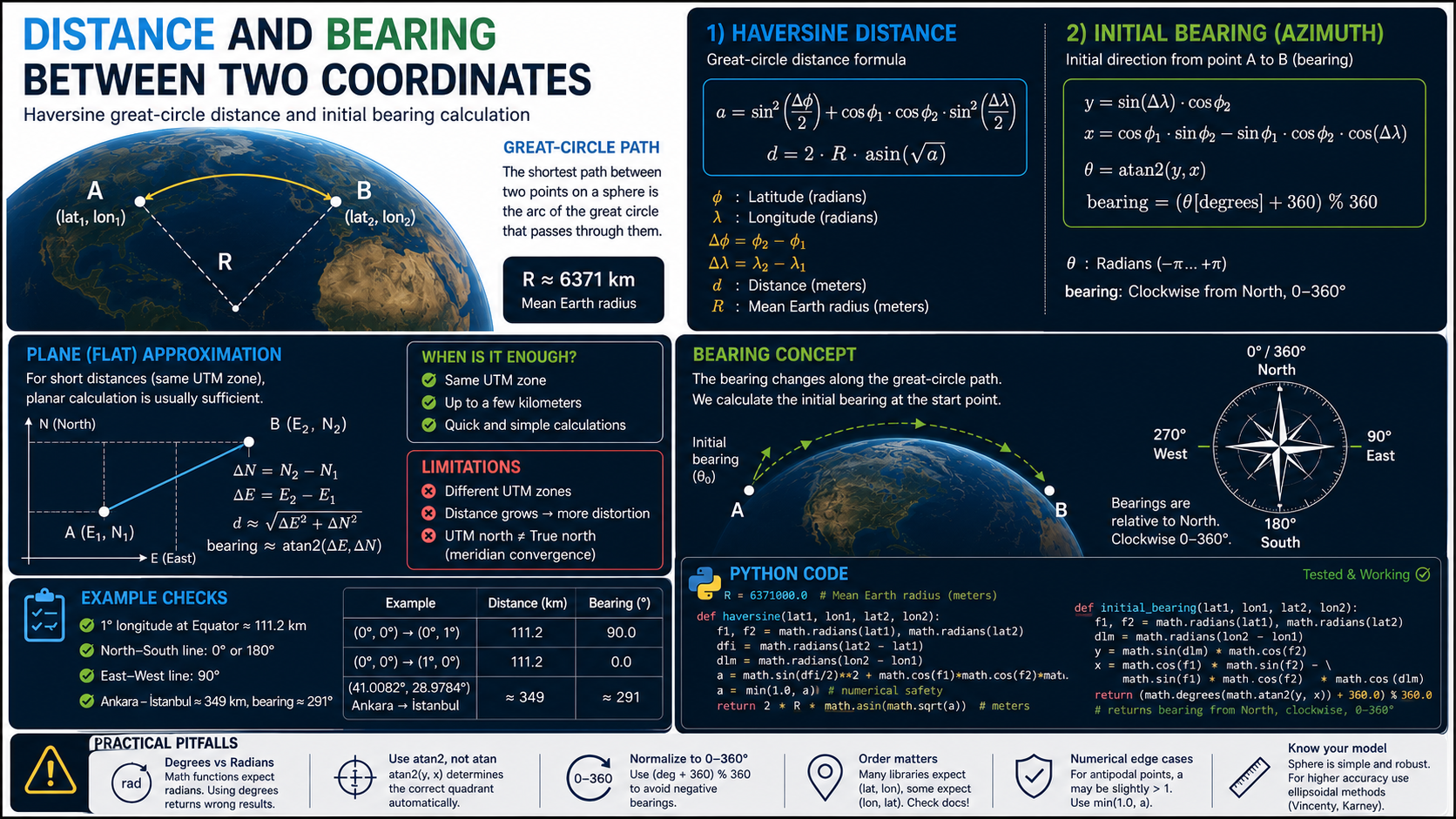
One of the calculations I run into most often when working with positioning systems is this: I have two latitude-longitude pairs, and I need to know the distance between them in meters and which direction to head. The question sounds simple, but the answer depends on which model of the Earth you accept. A flat sheet of paper? A sphere? An ellipsoid? In this post I'll explain the haversine formula, which works under the spherical assumption, along with the initial bearing calculation; then I'll cover when the planar approximation is good enough and when it misleads you. At the end there's tested Python code that does both calculations.
Great-circle distance with haversine
On a sphere, the shortest path between two points is the arc of the great circle passing through both. The haversine formula gives the length of that arc: an intermediate value is computed from the squared sines of half the latitude and longitude differences, and the distance is found as 2·R·asin(√a). For R, the Earth's mean radius of 6371 km is used. The formula's strong point is numerical stability; while the cosine-based spherical law of cosines loses precision at very short distances, haversine works cleanly even for differences of just a few meters. The cost is model error: the Earth isn't a sphere, it's the WGS84 ellipsoid. So haversine carries an error on the order of a few parts per thousand; over a 350-kilometer line, that can reach the order of a kilometer. It's more than sufficient for visualization and navigation; when I need geodetic precision, I switch to Vincenty or Karney (GeographicLib) methods.
Initial bearing: direction isn't a single number
As you travel along a great circle, your compass heading keeps changing; a flight from London to Tokyo departs heading northeast and lands heading southeast. That's why the direction between two points isn't actually a single number. What we compute is the initial bearing — the direction at the moment you set off. The formula uses atan2(y, x), where y is the trigonometric combination of the longitude difference and x is the trigonometric combination of the latitudes. The critical detail here is that atan2 returns a value in radians between -π and +π; converting with math.degrees brings that into the -180 to +180 degree range. Mapping applications, however, expect bearing in the 0-360 range, clockwise from north. The conversion is one line: (degrees + 360) % 360. If you forget this normalization, every route heading west comes out negative, and a value like -73° shows up in some corner of the interface.
When the planar approximation is enough
At small scale, the Earth's curvature isn't noticeable. If two points fall in the same UTM zone, their easting and northing coordinates are already in meters; you take the differences and apply the Pythagorean theorem, and atan2(ΔE, ΔN) suffices for the bearing. Over distances of a few kilometers, this approach gives practically the same result as haversine — and it's much easier to read and debug. In the desktop tools I work on, I usually choose this path for short distances.
Its limits are just as clear. If the points fall into different UTM zones, you can't compare the coordinates directly; as the distance grows into the tens of kilometers, projection distortion increases; and UTM's grid north isn't the same as true north. This difference, called meridian convergence, can reach 1-2 degrees at mid-latitudes near the edge of a zone. If an error of a few parts per thousand in distance, or one degree in bearing, matters for your application, it's time to move from the planar to the spherical calculation.
It's not enough for a formula to be correct; you also need to know which model of the Earth it assumes, and where that assumption breaks down.
import math
R = 6371000.0  # Dünya ortalama yarıçapı (metre)

def haversine(lat1, lon1, lat2, lon2):
    # Dereceleri radyana çevir, enlem ve boylam farklarını al
    f1, f2 = math.radians(lat1), math.radians(lat2)
    dfi, dlm = math.radians(lat2 - lat1), math.radians(lon2 - lon1)
    a = math.sin(dfi / 2) ** 2 + math.cos(f1) * math.cos(f2) * math.sin(dlm / 2) ** 2
    return 2 * R * math.asin(math.sqrt(a))  # büyük daire mesafesi, metre

def initial_bearing(lat1, lon1, lat2, lon2):
    # atan2 radyan döndürür (-pi..+pi); dereceye çevrilince -180..+180 olur, 0-360'a normalize ediyoruz
    f1, f2, dlm = math.radians(lat1), math.radians(lat2), math.radians(lon2 - lon1)
    y = math.sin(dlm) * math.cos(f2)
    x = math.cos(f1) * math.sin(f2) - math.sin(f1) * math.cos(f2) * math.cos(dlm)
return (math.degrees(math.atan2(y, x)) + 360.0) % 360.0 # kuzeyden saat yönünde- The math module expects radians; calling sin/cos with degrees doesn't raise an error, it silently produces a wrong result.
- Use atan2 instead of atan; because it evaluates signs separately, it finds the correct quadrant on its own.
- Normalize the bearing with (degrees + 360) % 360; -73 and 287 are the same direction but look different on screen.
- Watch the latitude-longitude order: some libraries expect (lat, lon), others (lon, lat); this is one of the sneakiest sources of error.
- Due to floating point, the value of a can exceed 1 by a hair's breadth; for points near the antipode, applying min(1.0, a) before sqrt is the safe practice.
After writing these two functions, I always test them against known values: a one-degree longitude difference at the equator should give about 111.2 km; a due north-south line should come out at 0° or 180°, and a due east line at 90°. Ankara to Istanbul should also come out at roughly 349 km and around 291°. I don't trust code that fails these checks; and even for code that passes, I trust it not blindly but knowing the limits of its model. Distance and bearing calculation is a small building block, but entire layers — route tracking, speed estimation, position verification — are built on top of it. It pays to get the foundation right.
